Functions calc_
functions_calc.Rmdcalc_ functions compute a certain value.
calc_acf
The goal of calc_acf is to compute the auto-correlation
function, given by:
$$\frac{\sum_\limits{t = k+1}^{n}(x_t - \bar{x})(x_{t-k} - \bar{x})}{\sum_\limits{t = 1}^{n} (x_t - \bar{x})^2 },$$ where:
- is a time series of length ;
- is a shifted time series by units in time;
- is the average of the time series.
calc_acf(x)
#> # A tibble: 21 × 2
#>        acf   lag
#>      <dbl> <dbl>
#>  1  1          0
#>  2 -0.0893     1
#>  3  0.0206     2
#>  4 -0.0172     3
#>  5 -0.136      4
#>  6 -0.0597     5
#>  7  0.0324     6
#>  8  0.169      7
#>  9 -0.0795     8
#> 10  0.0389     9
#> # ℹ 11 more rows
If you pass a second vector in the argument y the
cross-correlation will be computed instead:
$$\frac{n \left( \sum_\limits{t = 1}^{n}x_ty_t \right) - \left[\left(\sum_\limits{t = 1}^{n}x_t \right) \left(\sum_\limits{t = 1}^{n}y_t\right) \right]}{\sqrt{\left[n \left( \sum_\limits{t = 1}^{n}x_t^2 \right) - \left( \sum_\limits{t = 1}^{n}x_t \right)^2\right]\left[n \left( \sum_\limits{t = 1}^{n}y_t^2 \right) - \left( \sum_\limits{t = 1}^{n}y_t \right)^2\right]}},$$ where:
- is a time series of length ;
- is a time series of length .
calc_acf(x,y)
#> # A tibble: 33 × 2
#>        ccf   lag
#>      <dbl> <dbl>
#>  1  0.0755   -16
#>  2 -0.143    -15
#>  3  0.200    -14
#>  4 -0.234    -13
#>  5 -0.0297   -12
#>  6  0.0284   -11
#>  7  0.0534   -10
#>  8  0.111     -9
#>  9  0.0848    -8
#> 10 -0.179     -7
#> # ℹ 23 more rows
calc_association
The goal of calc_association is to compute associations
metrics.
Contingency
Contingency is a measure of the degree to which two nominal variables are associated. It has a value between 0 and 1, with 0 indicating no relationship and 1 indicating perfect association, and is calculated as follows:
where:
- the chi-square statistic;
- is the sample size.
calc_association(mtcars$am,mtcars$vs,type = "contingency")
#> [1] 0.1660092
Cramér’s V
Cramér’s V is a measure of the degree to which two nominal variables are associated. It has a value between 0 and 1, with 0 indicating no relationship and 1 indicating perfect association, and is calculated as follows:
where:
- the chi-square statistic;
- is the sample size;
- is the number of rows in the contingency table;
- is the number of columns in the contingency table.
calc_association(mtcars$am,mtcars$vs,type = "cramers-v")
#> [1] 0.1042136
Phi
Phi is a measure of association between two nominal dichotomous variables that takes into account a marginal table of the variables given by:
| y = 0 | y = 1 | Total | |
|---|---|---|---|
| x = 0 | |||
| x = 1 | |||
| Total |
Then the phi coefficient is given by:
calc_association(mtcars$am,mtcars$vs,type = "phi")
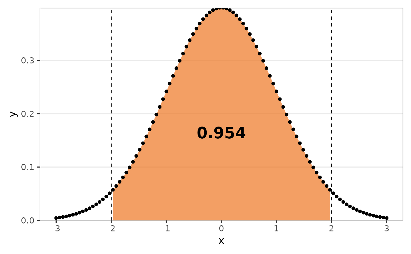
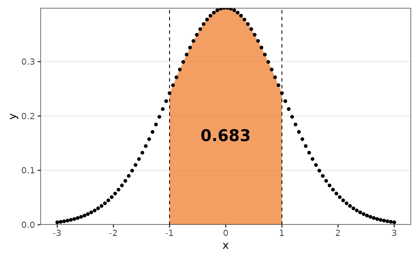
#> [1] 0.1700405calc_auc
The goal of calc_auc is to compute the area under a
curve (AUC).
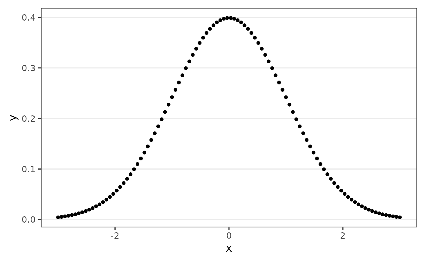
The function default compute the area considering the range of
x.
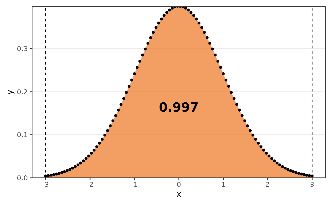
But you can define the argument limits to get the AUC of
that respective range.
calc_combination
The goal of calc_combination is to compute the number of
combinations/permutations. Given that there are a total of
observations and that
will be chosen.
Order matter with repetition
calc_combination(n = 10,r = 4,order_matter = TRUE,with_repetition = TRUE)
#> [1] 10000
Order matter without repetition
calc_combination(n = 10,r = 4,order_matter = TRUE,with_repetition = FALSE)
#> [1] 5040
Order does not matter with repetition
calc_combination(n = 10,r = 4,order_matter = FALSE,with_repetition = TRUE)
#> [1] 715
Order does not matter without repetition
calc_combination(n = 10,r = 4,order_matter = FALSE,with_repetition = FALSE)
#> [1] 210
calc_correlation
The goal of calc_correlation is to compute associations
metrics.
Kendall
The Kendall correlation coefficient, also known as the Kendall’s Tau coefficient, measures the relationship between two ranked variables.
Maurice Kendall created it, and it is especially useful for analyzing non-linear relationships or ranked data. The coefficient is calculated by counting the number of concordant pairs (ranks in the same order) and discordant pairs (ranks in opposite order) in the data.
where:
- is the number of concordant observations;
- is the number of discordant observations;
- is the number of observations.
calc_correlation(mtcars$hp,mtcars$drat,type = "kendall")
#> [1] -0.3826269
Pearson
The Pearson correlation coefficient quantifies the linear relationship that exists between two continuous variables. It ranges from -1 to 1, indicating the association’s strength and direction.
A value of 1 indicates a perfect positive linear relationship, a value of -1 indicates a perfect negative linear relationship, and a value of 0 indicates no linear relationship.
where:
- is the covariance of and ;
- is the variance of ;
- is the variance of .
calc_correlation(mtcars$hp,mtcars$drat,type = "pearson")
#> [1] -0.4487591
Spearman
The Spearman correlation coefficient assesses the strength and direction of a monotonic relationship between two variables, regardless of whether it is linear or non-linear.
It also has a value between -1 and 1, with 1 representing a perfect monotonic relationship and -1 representing a perfect inverse monotonic relationship. A value of 0 indicates that there is no monotonic relationship.
where:
- is the difference between the ranks of and ;
- is the number of observations.
calc_correlation(mtcars$hp,mtcars$drat,type = "spearman")
#> [1] -0.520125
calc_cv
The goal of calc_cv is to compute the coefficient of
variation (CV), given by:
where:
- is the sample standard deviation;
- is the sample mean.
If you set the argument as_perc to TRUE,
the CV will be multiplied by 100.
calc_cv(x,as_perc = TRUE)
#> [1] 99.32
calc_error
The goal of calc_error is to compute errors metrics.
Mean Absolute Error (MAE)
MAE measures the average absolute difference between the predicted and actual values:
Mean Absolute Percentage Error (MAPE)
MAPE measures the average percentage difference between the predicted and actual values relative to the actual values:
Mean Squared Error (MSE)
MSE measures the average of the squared differences between the predicted and actual values:
calc_kurtosis
The goal of calc_kurtosis is to compute a kurtosis
coefficient.
calc_kurtosis(x = x)
#> [1] -2.934065
Biased
The biased kurtosis coefficient, is given by:
where:
- is a numeric vector of length ;
- is the mean of ;
- is the standard deviation of .
calc_kurtosis(x = x,type = "biased")
#> [1] 14.81846
Excess
The excess kurtosis coefficient, is given by:
where:
- is a numeric vector of length ;
- is the mean of ;
- is the standard deviation of .
calc_kurtosis(x = x,type = "excess")
#> [1] 11.81846
Percentile
The percentile kurtosis coefficient, is given by:
where:
- is the first quartile;
- is the third quartile;
- is the 90th percentile;
- is the 10th percentile.
calc_kurtosis(x = x,type = "percentile")
#> [1] 0.3177264
Unbiased
The unbiased kurtosis coefficient, is given by:
where:
- is a numeric vector of length ;
- is the mean of ;
- is the standard deviation of .
calc_kurtosis(x = x,type = "unbiased")
#> [1] -2.934065
calc_mean
The goal of calc_mean is to compute the mean.
Arithmetic
Simple arithmetic mean
where:
- is a numeric vector of length .
calc_mean(x = 1:10,type = "arithmetic")
#> [1] 5.5
Weighted arithmetic mean
where:
- is a numeric vector of length ;
- is a numeric vector of length , with the respective weights of .
calc_mean(x = 1:10,type = "arithmetic",weight = 1:10)
#> [1] 7
Trimmed arithmetic mean
calc_mean(x = 1:10,type = "arithmetic",trim = .4)
#> [1] 5.5
Geometric
where:
- is a numeric vector of length .
calc_mean(x = 1:10,type = "geometric")
#> [1] 4.528729
Harmonic
where:
- is a numeric vector of length .
calc_mean(x = 1:10,type = "harmonic")
#> [1] 3.414172
calc_modality
The goal of calc_modality is to compute the number of
modes.
calc_modality(x = c("a","a","b","b"))
#> [1] 2
calc_mode
The goal of calc_mode is to compute the mode.
set.seed(123);cat_var <- sample(letters,100,replace = TRUE)

table(cat_var)
#> cat_var
#>  a  b  c  d  e  f  g  h  i  j  k  l  m  n  o  p  q  r  s  t  u  v  w  y  z
#>  1  2  5  2  4  3  6  4  5  4  3  3  3  6  4  3  3  3  4  3  4  8  3 10  4
We can see that the letter “y” appears the most, indicating that it is the variable’s mode.
calc_mode(cat_var)
#> [1] "y"
calc_peak_density
The goal of calc_peak_density is to compute the peak
density value of a numeric value.
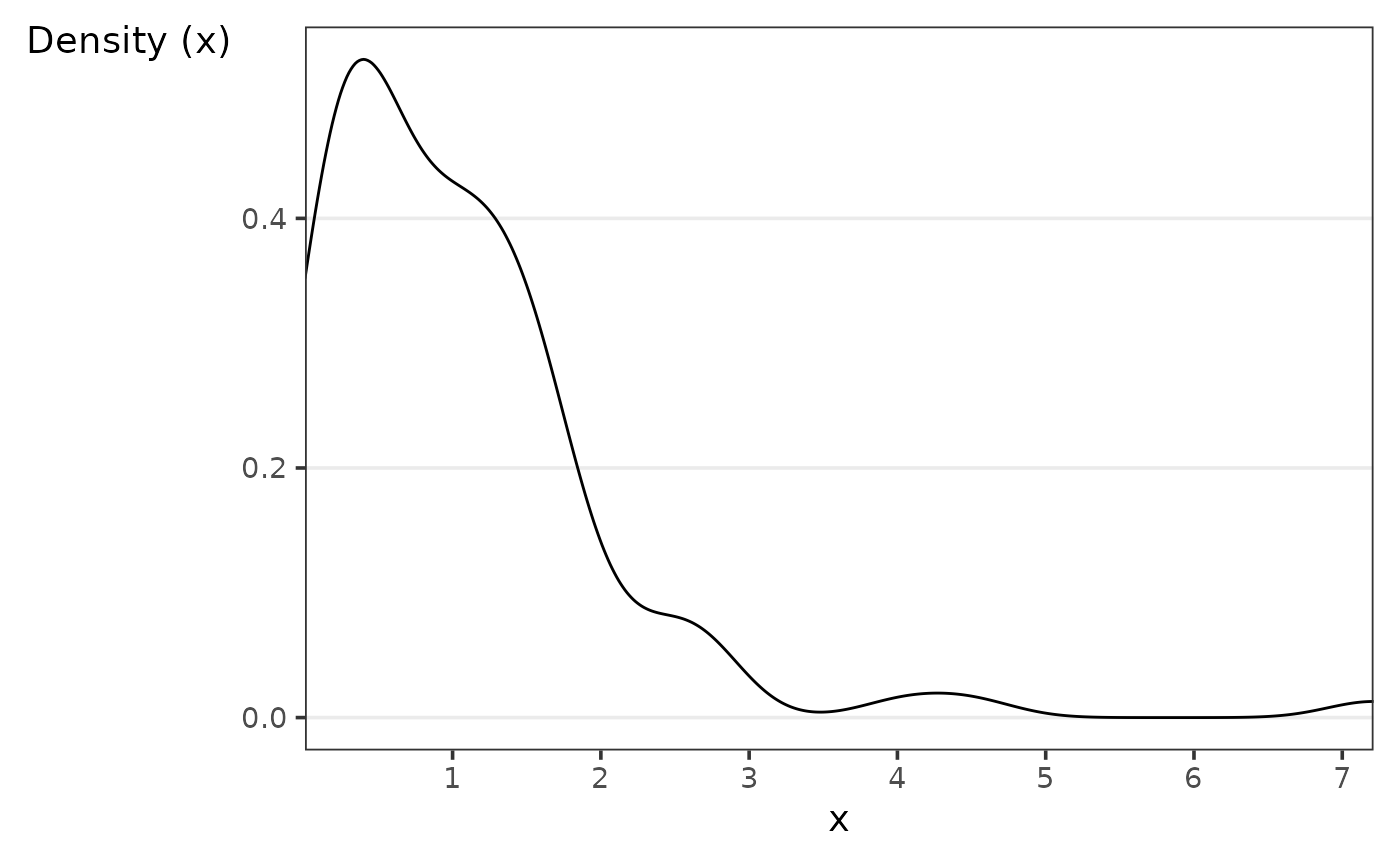
Assume we want to know what the density’s peak value is.
calc_peak_density(x)
#> [1] 0.3901813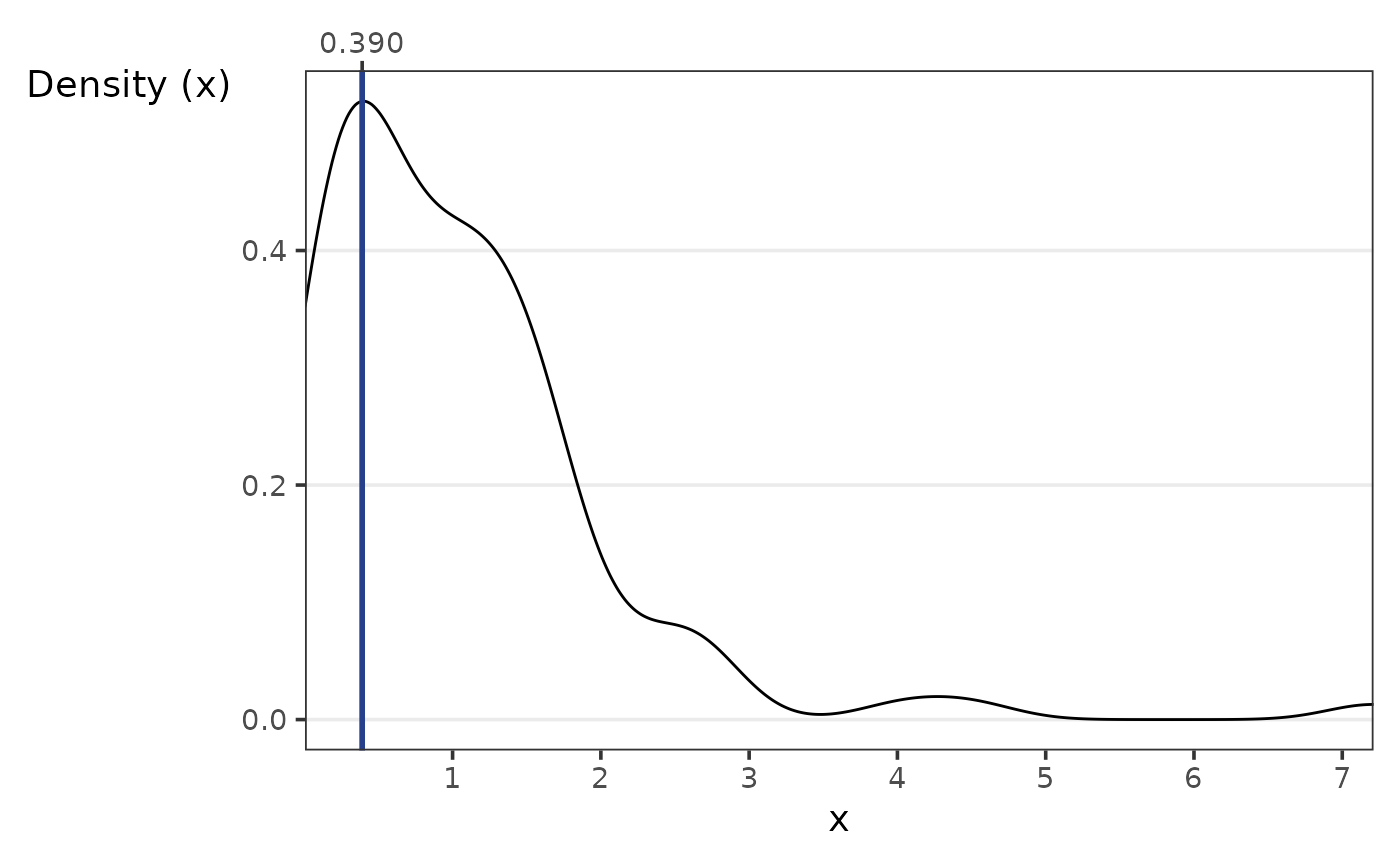
calc_perc
The goal of calc_perc is to compute the percentage.
#without main_var
calc_perc(mtcars,grp_var = c(cyl,vs))
#> # A tibble: 5 × 4
#>     cyl    vs     n  perc
#>   <dbl> <dbl> <int> <dbl>
#> 1     8     0    14 43.8
#> 2     4     1    10 31.2
#> 3     6     1     4 12.5
#> 4     6     0     3  9.38
#> 5     4     0     1  3.12

#main_var within grp_var
calc_perc(mtcars,grp_var = c(cyl,vs),main_var = vs)
#> # A tibble: 5 × 4
#> # Groups:   vs [2]
#>      vs   cyl     n  perc
#>   <dbl> <dbl> <int> <dbl>
#> 1     0     8    14 77.8
#> 2     0     6     3 16.7
#> 3     0     4     1  5.56
#> 4     1     4    10 71.4
#> 5     1     6     4 28.6

#main_var not within grp_var
calc_perc(mtcars,grp_var = c(cyl),main_var = vs)
#> # A tibble: 5 × 4
#> # Groups:   vs [2]
#>      vs   cyl     n  perc
#>   <dbl> <dbl> <int> <dbl>
#> 1     0     8    14 77.8
#> 2     0     6     3 16.7
#> 3     0     4     1  5.56
#> 4     1     4    10 71.4
#> 5     1     6     4 28.6
calc_skewness
The goal of calc_skewness is to compute a skewness
coefficient.
calc_skewness(x = x)
#> [1] 2.74827
Where different types of coefficients are provided, they are:
Bowley
The Bowley skewness coefficient, is given by:
where:
- is the first quartile;
- is the second quartile;
- is the third quartile.
calc_skewness(x = x,type = "bowley")
#> [1] 0.07563213
Fisher-Pearson
The Fisher-Pearson skewness coefficient, is given by:
$$\frac{\sum_\limits{i=1}^{n}(x_i - \bar{x})^3}{n*(s_x)^3},$$
where:
- is the mean of ;
- is a numeric vector of length ;
- is the standard deviation of .
calc_skewness(x = x,type = "fisher_pearson")
#> [1] 2.74827
Kelly
The Kelly skewness coefficient, is given by:
where:
- is the 90th percentile;
- is the second quartile, i.e., ;
- is the 10th percentile;
calc_skewness(x = x,type = "kelly")
#> [1] 0.1755126
Pearson median
The Pearson median skewness coefficent, or second skewness coefficient, is given by:
where:
- is the mean of ;
- is the median of ;
- is the standard deviation of .
calc_skewness(x = x,type = "pearson_median")
#> [1] 0.5718116
Rao
The Rao skewness coefficient, is given by:
where:
- is the mean of ;
- is the median of ;
- is the length of .
calc_skewness(x = x,type = "rao")
#> [1] 0.2019945