[1] 1 2 2 3 3 3 4 5 5 5 7| arithmetic |
|---|
| 3.636364 |
In this post, we will navigate the Land of the Averages.
The arithmetic mean, also known as “the mean,” is a fundamental concept in statistics that represents the average value of a set of numbers. It is widely used to summarize data in a variety of fields.
To calculate it, add up all of the numbers in a dataset and divide by the total count, yielding a central value that evenly distributes the data points on a number line.
The simple arithmetic mean, is given by: \[ \frac{1}{n}\sum_\limits{i=1}^{n} x_i, \tag{1}\]
where:
Because the arithmetic mean is simple to calculate and understand, it is accessible to a wide range of audiences, since it just entails the fundamental arithmetic operations of addition and division.
People frequently employ the concept, even if they do not formally comprehend it. In my classes, I used to ask how long it usually takes you to get to work. Then someone said they’d take 30 minutes, for example, and I asked if that meant every day would be exactly 30 minutes, and my students said no, that some times would be 30, 31 or 29 minutes, so intuitively they’d do the simple arithmetic mean.
[1] 1 2 2 3 3 3 4 5 5 5 7| arithmetic |
|---|
| 3.636364 |
So the simple arithmetic mean is 3.636364, now let’s see how outliers impact.
In this example, we change the first value to a smaller fractional value.
[1] 0.1 2.0 2.0 3.0 3.0 3.0 4.0 5.0 5.0 5.0 7.0| arithmetic |
|---|
| 3.554546 |
We can see that the mean has shifted slightly to a smaller value.
The arithmetic mean can be significantly influenced by extreme values. A single value that is unusually high or low can skew the result, resulting in an inaccurate representation of the central tendency. Extreme values in small samples can have a greater impact on the mean than extreme values in large samples.
Now we change the last value to a larger value.
[1] 1 2 2 3 3 3 4 5 5 5 100| arithmetic |
|---|
| 12.09091 |
As we can see, the mean increases significantly, resulting in a distorted and unrepresentative metric of the data.
In skewed distributions, the mean may not accurately represent the typical value experienced by the majority of data points. The mean can be pushed towards the distribution’s tail.
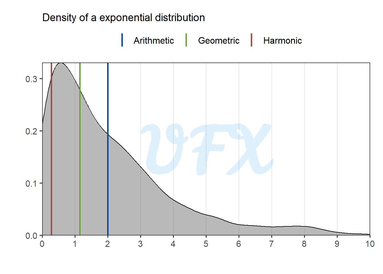
Let’s take a look at an example from a dataset from a exponential distribution.
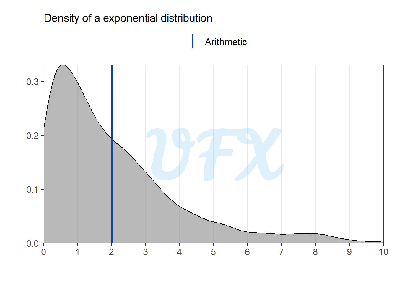
As we can see, the mean is dragged far away from the peak density value by the larger values.
Next we apply the mean to data from a normal distribution centered around zero.
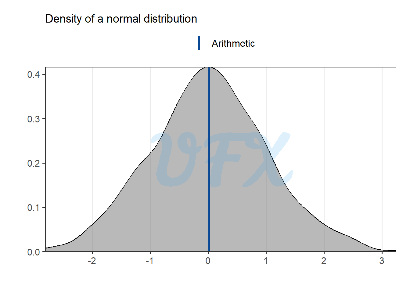
Because the arithmetic mean uses sum as the base for calculation, a simmetric distribution around negative and positive values will produce a mean close to or equal to zero, which can be misleading, especially when dealing with an error variable, because the mean can be interpreted as having no error at all, which is why the absolute function is commonly used in this scenario.
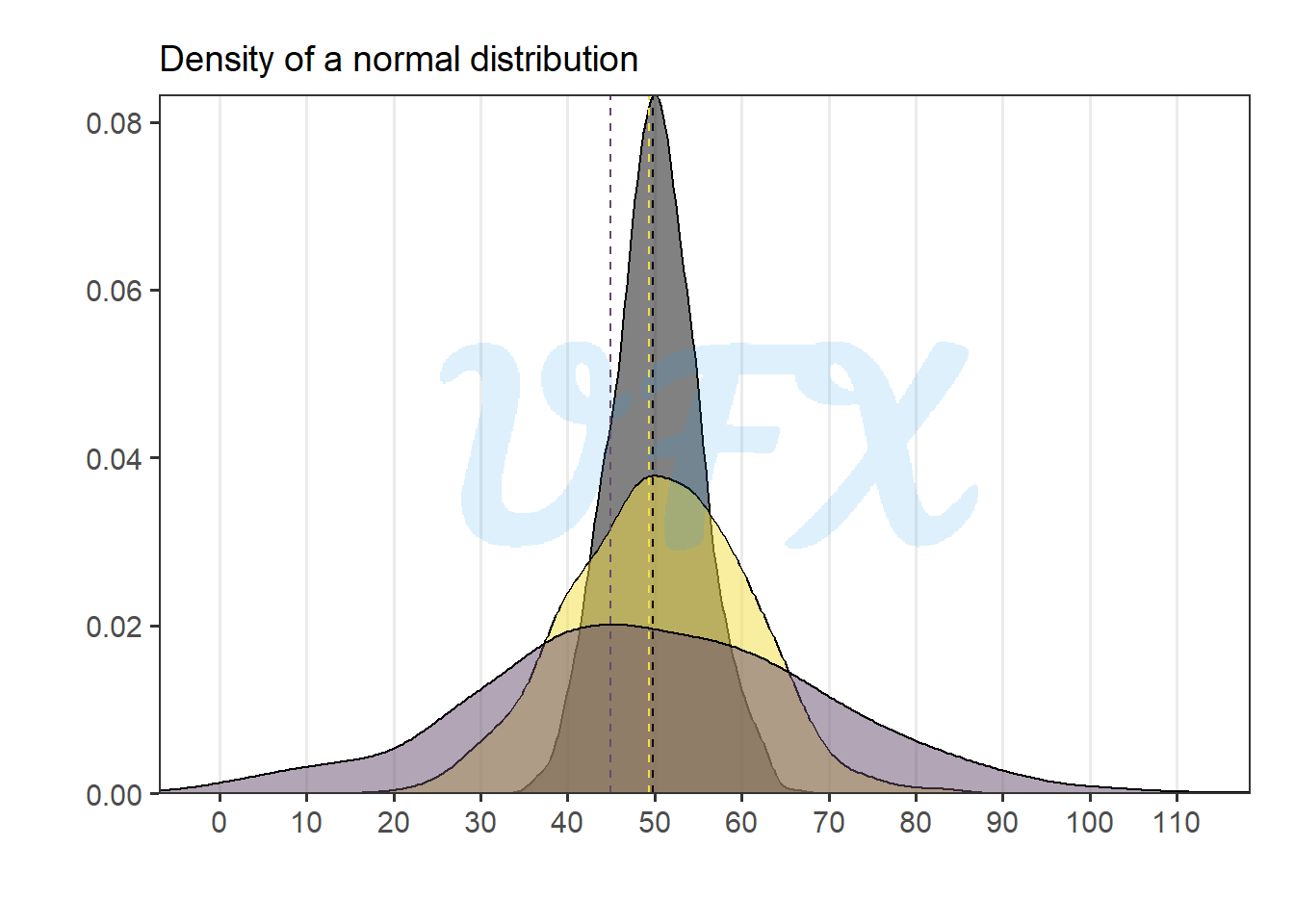
Let’s run the normal distribution simulation again, but with different variances this time.

We can see that even though the distribution for each data set is very different, we would be in trouble if we only based our decision on the mean.
The weighted arithmetic mean is a variant that considers not only the values in a dataset but also assigns different weights to each value based on its importance or significance.
In other words, rather than treating all values equally, the weighted mean favors some over others based on predetermined weights.
\[ \frac{1}{\sum_\limits{i=1}^{n}w_i}\sum_\limits{i=1}^{n} w_ix_i, \tag{2}\]
where:
\(x_i\) is a numeric vector of length \(n\);
\(w_i\) is a numeric vector of length \(n\), with the respectives weights for the values of \(x_i\).
A practical application is in academic grading, the weighted mean of exam scores might be used, where different exams carry different weights based on their importance.
A common case is when proportion (\(p_i\)) are used as weigths, and since:
\[ \sum_\limits{i=1}^{n} p_i = 1. \tag{3}\]
When applying Equation 3 to Equation 2 we have that:
\[ \sum_\limits{i=1}^{n} w_ix_i. \tag{4}\] Even if it is an interesting application, assigning weights to data points is frequently subjective and can be influenced by personal judgment or assumptions. The weighted mean’s accuracy is heavily dependent on the appropriateness of the weights chosen.
In addition, calculating the weighted mean requires an extra step when compared to the simple arithmetic mean, which may complicate the analysis and calculations, particularly when dealing with large datasets. In some cases, the rationale for assigning specific weights may not be transparent or well-documented, which can make replicating or validating the analysis difficult.
A trimmed arithmetic mean is a statistical measure that computes the mean of a dataset by excluding a percentage of the lowest and highest values, reducing the impact of outliers and extreme values.
The amount of trimming can be adjusted to strike a balance between retaining meaningful data and reducing the impact of outliers.
Let’s go back to our previous outlier example, but now applying a trim of 10% in both ends of the data.
[1] 1 2 2 3 3 3 4 5 5 5 100| trimmed |
|---|
| 3.555556 |
That is the same as applying a simple arithmetic mean to:
[1] 2 2 3 3 3 4 5 5 5| arithmetic |
|---|
| 3.555556 |
As the data is trimmed, we achieve a more representative metric for our data, but this is due to an intentional loss of information, which may result in an incomplete representation of the data’s full range. Important insights or trends within the data may be overlooked depending on the extent of trimming.
The geometric mean is a statistical measure used to determine the central tendency of a set of values, particularly when those values are multiplicatively related.
The geometric mean, as opposed to the arithmetic mean, involves multiplying the values and then taking the \(n\)th root, where \(n\) is the total number of values. This makes it especially useful for data with exponential or multiplicative growth, such as investment returns, population growth rates, or scientific measurements.
\[ \sqrt[n]{\prod_\limits{i=1}^{n} x_i}, \tag{5}\]
where:
Another way to write the Equation 5 is:
\[ \begin{align} \sqrt[n]{\prod_\limits{i=1}^{n} x_i} &= \sqrt[n]{x_1x_2...x_n} \\ &= (x_1x_2...x_n)^{1/n} \\ &= \mathcal{e}^{\mathcal{ln}(x_1x_2...x_n)^{1/n}}\\ &= \mathcal{e}^{\frac{1}{n}[\mathcal{ln}(x_1)+\mathcal{ln}(x_2)...+\mathcal{ln}(x_n) ]}\\ &= \mathcal{e}^{\frac{1}{n}\sum_\limits{i=1}^{n}\mathcal{ln}(x_i)}. \end{align} \tag{6}\]
So we can see that the geometric mean can be written as the exponential of the simple arithmetic mean (Equation 1) of the logarithmic of \(x_i\).
Let’s go back to our first example and see in comparison to the arithmetic mean.
[1] 1 2 2 3 3 3 4 5 5 5 7| arithmetic | geometric |
|---|---|
| 3.636364 | 3.213991 |
We can see that the geometric mean yields a slightly lower value. When using the geometric mean with fractional values, the result represents the “average growth factor” between the values. It indicates the factor by which you need to multiply each value to obtain the overall product.
[1] 0.100 0.200 0.300 0.050 0.004| arithmetic | geometric |
|---|---|
| 0.1308 | 0.0654389 |
The geometric mean is sensitive to small values in the dataset. This sensitivity can be advantageous when you want to emphasize the impact of small values or identify trends that might be overshadowed by larger values.
[1] 0.1 2.0 2.0 3.0 3.0 3.0 4.0 5.0 5.0 5.0 7.0| arithmetic | geometric |
|---|---|
| 3.554546 | 2.606968 |
As we can see, the presence of the smaller value severely “penalizes” the geometric value.
Unlike the arithmetic mean, the geometric mean is less affected by larger outliers. This is due to the fact that the geometric mean is equivalent to taking the arithmetic mean of the logarithms of the values. This property has the effect of compressing the data, making extreme values contribute less to the final result.
Let’s go back to our outlier example.
[1] 1 2 2 3 3 3 4 5 5 5 100| arithmetic | geometric |
|---|---|
| 12.09091 | 4.092944 |
As we can see, the geometric mean has a significant less impact of the larger value.
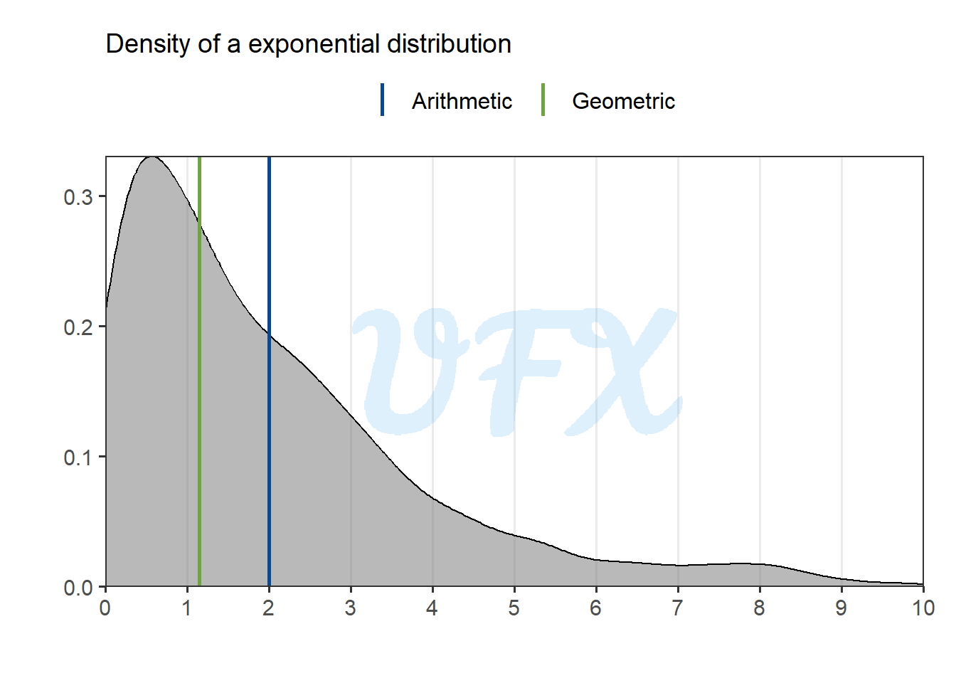
In this scenario, the geometric mean approaches the peak value of the density in the example because it is more resistant to larger values and more sensitive to smaller data.
When a zero value is present in a dataset, calculating the geometric mean becomes problematic because the value will always be zero, since it is the product of values.
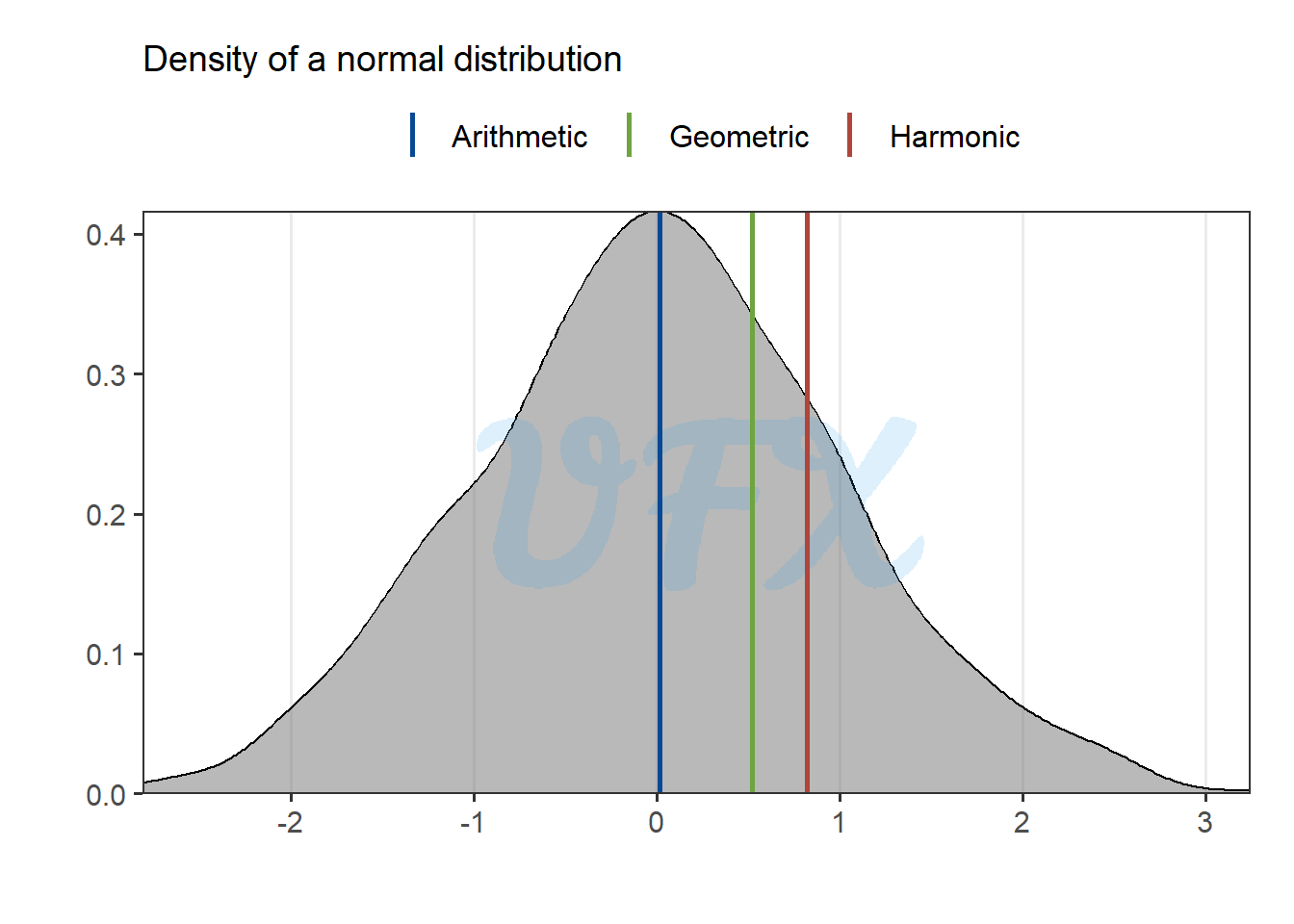
But let’s take a look in our previous example where the data follows a normal distribution around zero.
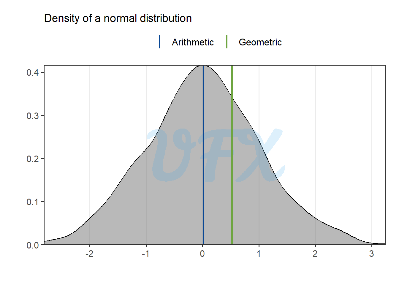
The geometric mean results in value larger than zero, that is because it does not consider negative values, because a negative number raised to a non-integer exponent can produce complex results, the concept of a geometric mean for negative values is meaningless in the realm of real numbers.
Let’s run the normal distribution again, but this time with different variances.
We get a similar result, but in the higher variance distribution, the mean becomes more skewed toward the peak density.
The harmonic mean is a statistical measure of central tendency used to calculate the average of a set of values when their reciprocal (inverses) is more important than their arithmetic mean.
\[ \frac{n}{\sum_\limits{i=1}^{n}\frac{1}{x_i}}, \tag{7}\]
where:
Let’s compare it to the other approaches.
[1] 1 2 2 3 3 3 4 5 5 5 7| arithmetic | geometric | harmonic |
|---|---|---|
| 3.636364 | 3.213991 | 2.75492 |
We can see that harmonic provided a smaller value to our fist example.
Since the harmonic mean takes the inverse of the original value, it is even more sensitive to small values than the geometric mean, leading to extremely large results for values close to zero.
[1] 0.1 2.0 2.0 3.0 3.0 3.0 4.0 5.0 5.0 5.0 7.0| arithmetic | geometric | harmonic |
|---|---|---|
| 3.554546 | 2.606968 | 0.846619 |
Next, we see how it is impacted by a larger value.
[1] 1 2 2 3 3 3 4 5 5 5 100| arithmetic | geometric | harmonic |
|---|---|---|
| 12.09091 | 4.092944 | 2.849741 |
At the same time that it is most sensitive to small values, it is also the most robust to larger values.
Because the harmonic mean is more robust to larger values and more sensitive to smaller data, it provides a lower value in the example above than the other methods.
Calculating the harmonic mean when there is a zero value in a dataset becomes difficult because the value is undefined since it is the sum of the inverse of the values and there is no division by zero.
But let’s take a look in our previous example where the data follows a normal distribution around zero.
Because we are using a dataset with a small magnitude, the harmonic mean provides a value that is even further away from the center than the geometric mean.
Let’s run the normal distribution again, but this time with different variances.

The harmonic mean achieves nearly the same result as the arithmetic mean, where the metrics are all centered around 50 when the variance is ignored.
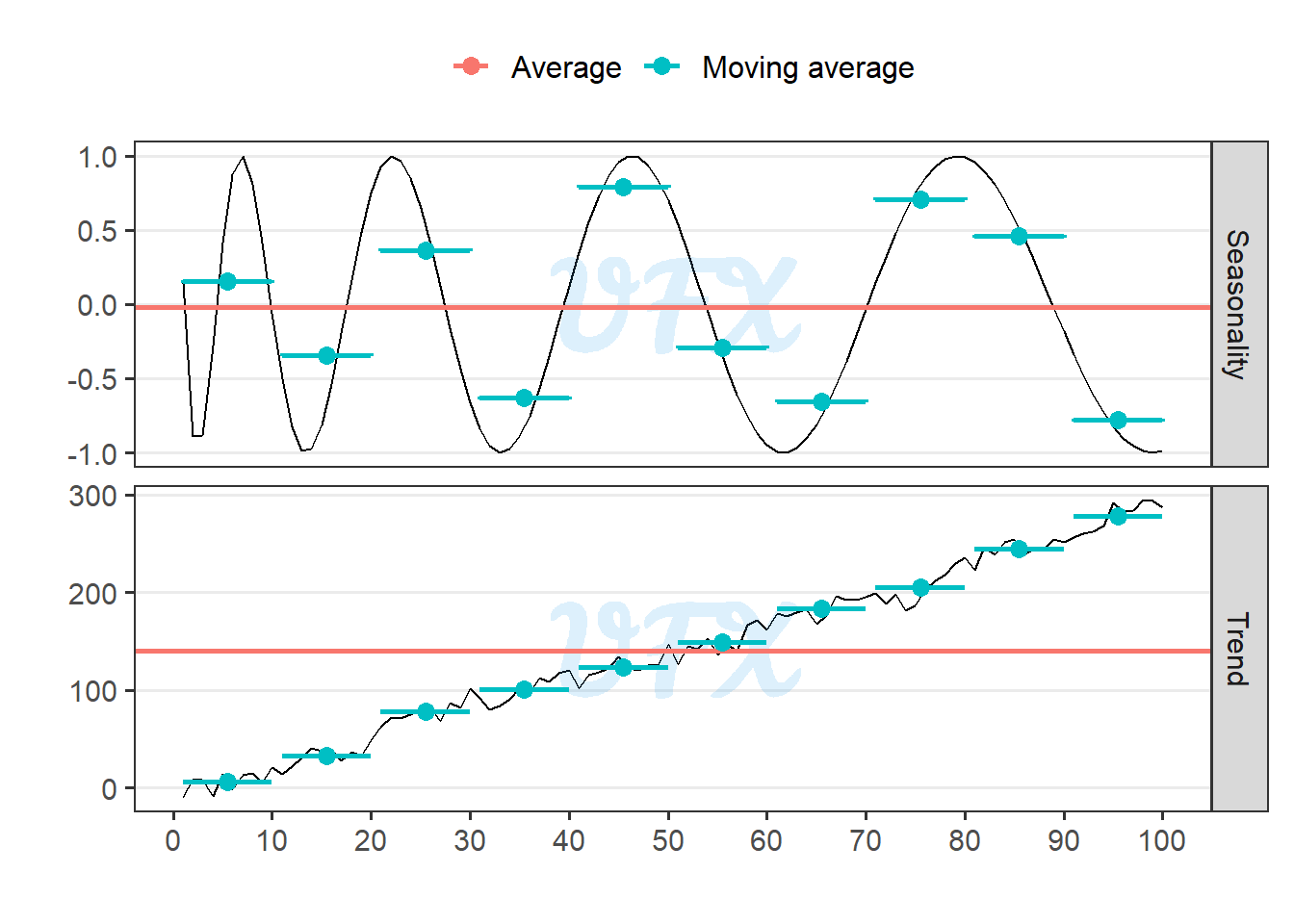
In time series we can have some special patterns in data, the two most common are trends, which represent long-term consistent movements in data, whether upward, downward, or flat, and seasonality, which refers to recurring and predictable patterns that repeat at regular intervals, linked to specific calendar periods.
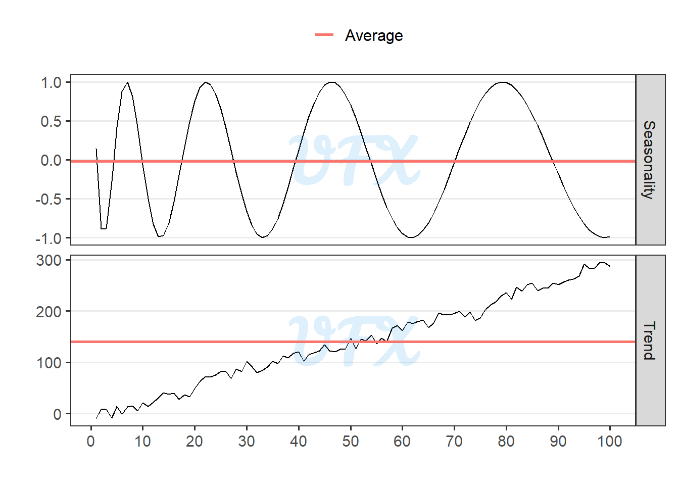
When the mean is applied to the entire period, the result can be meaningless. So, how do we arrive at a representative metric?
A moving average is a statistical technique used to smooth out fluctuations in time series or sequential data by averaging a subset of data points within a moving window. It reduces noise to reveal underlying trends and patterns, and it is available in a variety of forms, including the simple moving average, weighted moving average, and exponential moving average.
To use the moving average, we must first define the interval over which the average will be calculated; in the example below, we will first display the moving average for each 10 units of time.
The moving average can improve data smoothing, noise reduction, and trend identification by highlighting underlying patterns by averaging subsets of data points. However, due to the equal weighting of all data points, it introduces a lag in detecting rapid changes, is sensitive to window size, and may not accurately capture recent trends.
While moving averages are effective for regular patterns, they may be ineffective for irregular data or abrupt shifts, potentially leading to oversimplification and loss of detail in the analysis. Because of the lag in detecting rapid changes and the potential impact of outliers, the moving average type and window size should be chosen based on data characteristics and analysis objectives.
In R we have the mean function that compute the simple arithmetic mean, and also we have the trim argument to compute the trimmed arithmetic mean. Also we have the weighted.mean where we can pass the weights in the w argument to compute the weighted arithmetic mean.
However, there is no native way to compute the geometric or hamonic means, so I created a function in my package relper that encompasses all possibilities.
x <- c(.001,2,2,2,2,2,3,3,4,4,4,5,5,5,5,70)

#simple arithmetic mean
relper::calc_mean(x = x,type = "arithmetic")
[1] 7.375063#weighted arithmetic mean
relper::calc_mean(x = x,type = "arithmetic",weight = 1:16)[1] 11.72795#trimmed arithmetic mean
relper::calc_mean(x = x,type = "arithmetic",trim = .1)[1] 3.6#geometric mean
relper::calc_mean(x = x,type = "geometric")[1] 2.339696#trimmed geometric mean
relper::calc_mean(x = x,type = "geometric",trim = .1)[1] 3.565205#harmonic mean
relper::calc_mean(x = x,type = "harmonic")[1] 0.01592466#trimmed harmonic mean
relper::calc_mean(x = x,type = "harmonic",trim = .1)[1] 3.529412