In this post, we explore the infamous metric R².
Context
The R² or the coefficient of determination is a metric commonly used to measure the goodness of fit of a model, it is given by:
\[ R^2 = 1- \frac{SS_{\mathrm{res}}}{SS_{\mathrm{tot}}}, \tag{1}\]
where:
\(SS_{\mathrm{res}}\) is the sum of squares of residuals;
\(SS_{\mathrm{tot}}\) is the total sum of squares.
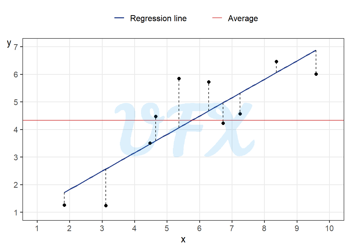
The sum of squares of residuals is given by: \[ SS_{\mathrm{res}} = \sum_\limits{i=1}^{n}(y_i - \hat{y}_i)^2, \tag{2}\]
where:
\(y_i\) is the response variable;
\(\hat{y}_i\) is the fitted value for \(y_i\).
The graphic below shows the difference between the original values and the model (\(y_i - \hat{y}_i\)).
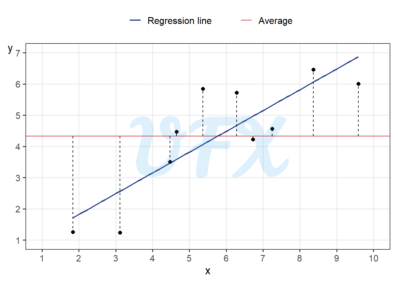
The total sum of squares is given by: \[ SS_{\mathrm{tot}} = \sum_\limits{i=1}^{n}(y_i - \bar{y})^2, \tag{3}\]
where:
\(y_i\) is the response variable;
\(\bar{y}\) is the average value of \(y\).
The graphic below shows the difference between the response variable’s original values and its mean (\(y_i - \bar{y}\)).
To put it simply, the coefficient measures the relative difference between the sum of squares of your model compared to a simplistic model (the average), where its values is considered good if it equals 1, meaning that the \(SS_{\mathrm{res}}\) is close to 0 and is considered bad as it approaches 0, since the squared sum of the residuals would be close as using the average as a model.
When R² = (r)²?
A well-known fact is that for simple linear regression, we have a direct relationship between the coefficient of determination and the Pearson linear correlation coefficient. To show the relationship between the \(R^2\) and \(r\) , first we have that
\[ SS_{\mathrm{tot}} = SS_{\mathrm{res}} + SS_{\mathrm{reg}}. \tag{4}\]
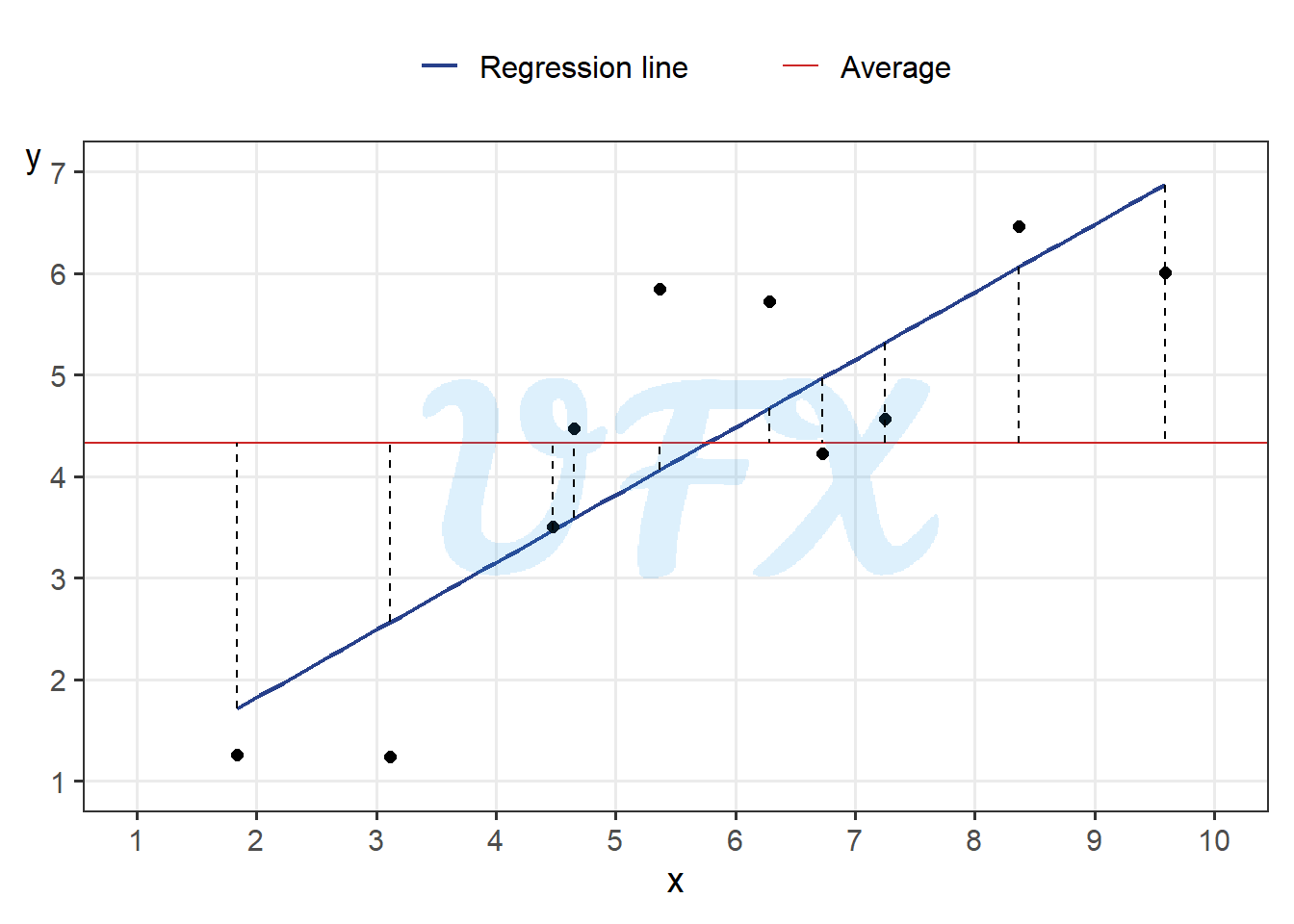
where \(SS_{\mathrm{reg}}\) is the sum of squares due to regression, also known as the explained sum of squares, giving by:
\[ SS_{\mathrm{reg}} = \sum_\limits{i=1}^{n}(\hat{y}_i - \bar{y})^2. \tag{5}\]
Or graphically,
Then, applying the Equation 4 to the Equation 1 :
\[ \begin{align} R^2 &= 1- \frac{SS_{\mathrm{res}}}{SS_{\mathrm{tot}}}\\ &= \frac{SS_{\mathrm{tot}}}{SS_{\mathrm{tot}}}- \frac{SS_{\mathrm{res}}} {SS_{\mathrm{tot}}}\\ &= \frac{SS_{\mathrm{tot}} - SS_{\mathrm{res}}}{SS_{\mathrm{tot}}}\\ &= \frac{SS_{\mathrm{reg}} + \cancel{{SS_{\mathrm{res} } - SS_{\mathrm{res}}}}}{SS_{\mathrm{tot}}}\\ &= \frac{SS_{\mathrm{reg}}}{SS_{\mathrm{tot}}}.\\ \end{align} \tag{6}\]
So with the Equation 5 applied to the Equation 6, we have that
\[ \begin{align} R^2 &= \frac{SS_{\mathrm{reg}}}{SS_{\mathrm{tot}}}\\ &= \frac{\sum_\limits{i=1}^{n}(\hat{y}_i - \bar{y})^2}{ \sum_\limits{i=1}^{n}(y_i - \bar{y})^2}. \end{align} \tag{7}\]
For a simple linear regression, we can compute the fitted value as
\[ \hat{y}_i = \hat{\beta}_0 + \hat{\beta}_1x_i, \tag{8}\]
where:
\(\hat{\beta}_0\) is the estimated value of the intercept;
\(\hat{\beta}_1\) is the estimated value of the slope coefficient;
\(x_i\) is the explanatory variable.
Applying the Equation 8 in the Equation 7 we have that
\[ \begin{align} R^2 &= \frac{\sum_\limits{i=1}^{n}(\hat{y}_i - \bar{y})^2}{ \sum_\limits{i=1}^{n}(y_i - \bar{y})^2}\\ &= \frac{\sum_\limits{i=1}^{n}(\hat{\beta}_0 + \hat{\beta}_1x_i - \bar{y})^2}{ \sum_\limits{i=1}^{n}(y_i - \bar{y})^2}. \end{align} \tag{9}\]
We also have a result for the ordinary least squares of the simple linear regresson that:
\[ \hat{\beta}_0 = \bar{y} - \hat{\beta}_1\bar{x}. \tag{10}\]
So the Equation 10 applied to the Equation 9 results in:
\[ \begin{align} R^2 &= \frac{\sum_\limits{i=1}^{n}(\hat{\beta}_0 + \hat{\beta}_1x_i - \bar{y})^2}{ \sum_\limits{i=1}^{n}(y_i - \bar{y})^2}\\ &= \frac{\sum_\limits{i=1}^{n}(\cancel{\bar{y}} - \hat{\beta}_1\bar{x} + \hat{\beta}_1x_i \cancel{-\bar{y}})^2}{ \sum_\limits{i=1}^{n}(y_i - \bar{y})^2}\\ &= \frac{\sum_\limits{i=1}^{n}(- \hat{\beta}_1\bar{x} + \hat{\beta}_1x_i)^2}{ \sum_\limits{i=1}^{n}(y_i - \bar{y})^2}\\ &= \frac{\sum_\limits{i=1}^{n}[\hat{\beta}_1 (x_i- \bar{x})]^2}{ \sum_\limits{i=1}^{n}(y_i - \bar{y})^2}\\ &= \frac{\sum_\limits{i=1}^{n}\hat{\beta}^2_1(x_i- \bar{x})^2}{ \sum_\limits{i=1}^{n}(y_i - \bar{y})^2}\\ &= \hat{\beta}^2_1\left(\frac{\sum_\limits{i=1}^{n}(x_i- \bar{x})^2}{ \sum_\limits{i=1}^{n}(y_i - \bar{y})^2}\right). \end{align} \tag{11}\]
Since we have that the variance of \(x\) is given by
\[ s^2_x = \frac{1}{n-1}\sum_\limits{i=1}^{n}(x_i- \bar{x})^2. \tag{12}\]
We can divide both terms of the Equation 11 by \((n-1)\) and use the Equation 12 to rewrite it as
\[ \begin{align} R^2 &= \hat{\beta}^2_1\left(\frac{\frac{1}{n-1}\sum_\limits{i=1}^{n}(x_i- \bar{x})^2}{\frac{1}{n-1} \sum_\limits{i=1}^{n}(y_i - \bar{y})^2}\right)\\ &= \hat{\beta}^2_1\frac{s^2_x}{s^2_y}\\ &= \left(\hat{\beta}_1\frac{s_x}{s_y}\right)^2.\\ \end{align} \tag{13}\]
Such as we have a result for \(\hat{\beta}_0\) in the Equation 10, we also have one for \(\hat{\beta}_1\)
\[ \hat{\beta}_1 = \frac{s_{xy}}{s^2_x}, \tag{14}\]
where
- \(s_{xy}\) is the covariance between \(x\) and \(y\).
Finally, applying the Equation 14 to the Equation 13
\[ \begin{align} R^2 &= \left(\hat{\beta}_1\frac{s_x}{s_y}\right)^2\\ &= \left(\frac{s_{xy}}{s^2_x}\frac{s_x}{s_y}\right)^2\\ &= \left(\frac{s_{xy}}{s_xs_y}\right)^2\\ &= (r)^2.\\ \end{align} \tag{15}\]
At last in Equation 15 we can show that for the simple linear regression that \(R^2 = (r)^2\).
Adjusted R²
Another version of R², is the ajusted version, where it tries to correct the overestimation, by penalizing the number of variables used in the model.
To attempt that, instead of only the sum of squares we divide the terms by their respectives degrees of freedom:
\[ \frac{SS_{\mathrm{tot}}}{n-1}, \tag{16}\]
and
\[ \frac{SS_{\mathrm{res}}}{n-p-1}, \tag{17}\]
where
- \(p\) is the number of explanatory variables.
Then using both Equation 16 and Equation 17 applied to Equation 1 we can compute the adjusted version:
\[ \begin{align} R^2_{\mathrm{adj}} &= 1 - \frac{\frac{\sum_\limits{i=1}^{n}(y_i - \hat{y}_i)^2}{n-p-1}}{\frac{\sum_\limits{i=1}^{n}(y_i - \bar{y})^2}{n-1}}\\ &= 1 - \left(\frac{\sum_\limits{i=1}^{n}(y_i - \hat{y}_i)^2}{\sum_\limits{i=1}^{n}(y_i - \bar{y})^2}\right) \left(\frac{n-1}{n-p-1}\right)\\ &= 1 - \left(1- R^2\right) \left(\frac{n-1}{n-p-1}\right). \end{align} \tag{18}\]
Why it can be a poor choice
Despite being one of the most well-known metrics in modeling, it is also one of the most criticized, for a variety of reasons, such as:
Can be arbitrarily low even if the model follows the assumptions and makes sense; similarly, it can be arbitrarily close to 1 when the model is erroneous. A good example is when nonlinear models achieve a high R² for linear data;
Sensitivity to the number of predictors, which increases with the number of predictors, even if the predictors are irrelevant to the outcome. As we saw earlier, the adjusted version helps to mitigate this issue;
Because it relies primarily on the mean, outliers can have a substantial impact, making it also a poor prediction indication since it compares your model’s error to the error of the average model;
It cannot be compared across datasets since it can only be compared when several models are fitted to the same data set with the same untransformed response variable.
For more details on the points above: