In this post you will learn what bell, Gauss and simmetry have in common.
Introduction
A probability distribution is a function that describes the likelihood of various outcomes in a random event. It assigns probabilities to each possible outcome, indicating how likely each is.
In statistics the normal distribution holds the most popular position of distributions. It has many names, such as:
Bell curve;
Gaussian distribution;
Laplace-Gauss distribution.
The term “normal” does not mean “typical” or “ordinary” in this context, but stems from the Latin word normalis, which means “perpendicular” or “at right angles.”
Due to its mathematical properties, symmetry, and prevalence in nature and various phenomena, Carl Friedrich Gauss named it the normal distribution, in the 19th century.
Math
A Normal distribution possess two parameters, the mean (\(\mu\)) and the standard deviation (\(\sigma\)), so we can describe a variable \(X\) following a normal distribution as \(X \sim \mathcal{N}(\mu,\sigma)\):
\[ f(x) = \frac{1}{\sigma\sqrt{2\pi}}\mathcal{e}^{-\frac{1}{2}\left(\frac{x-\mu}{\sigma}\right)^2}. \tag{1}\]
Standard normal
The simplest case of a normal distribution is a \(\mathcal{N}(0,1)\), also called a standard normal distribution or Z-distribution:
\[ f(x) = \frac{1}{\sqrt{2\pi}}\mathcal{e}^{-\frac{x^2}{2}}. \tag{2}\]
Properties
Simmetry
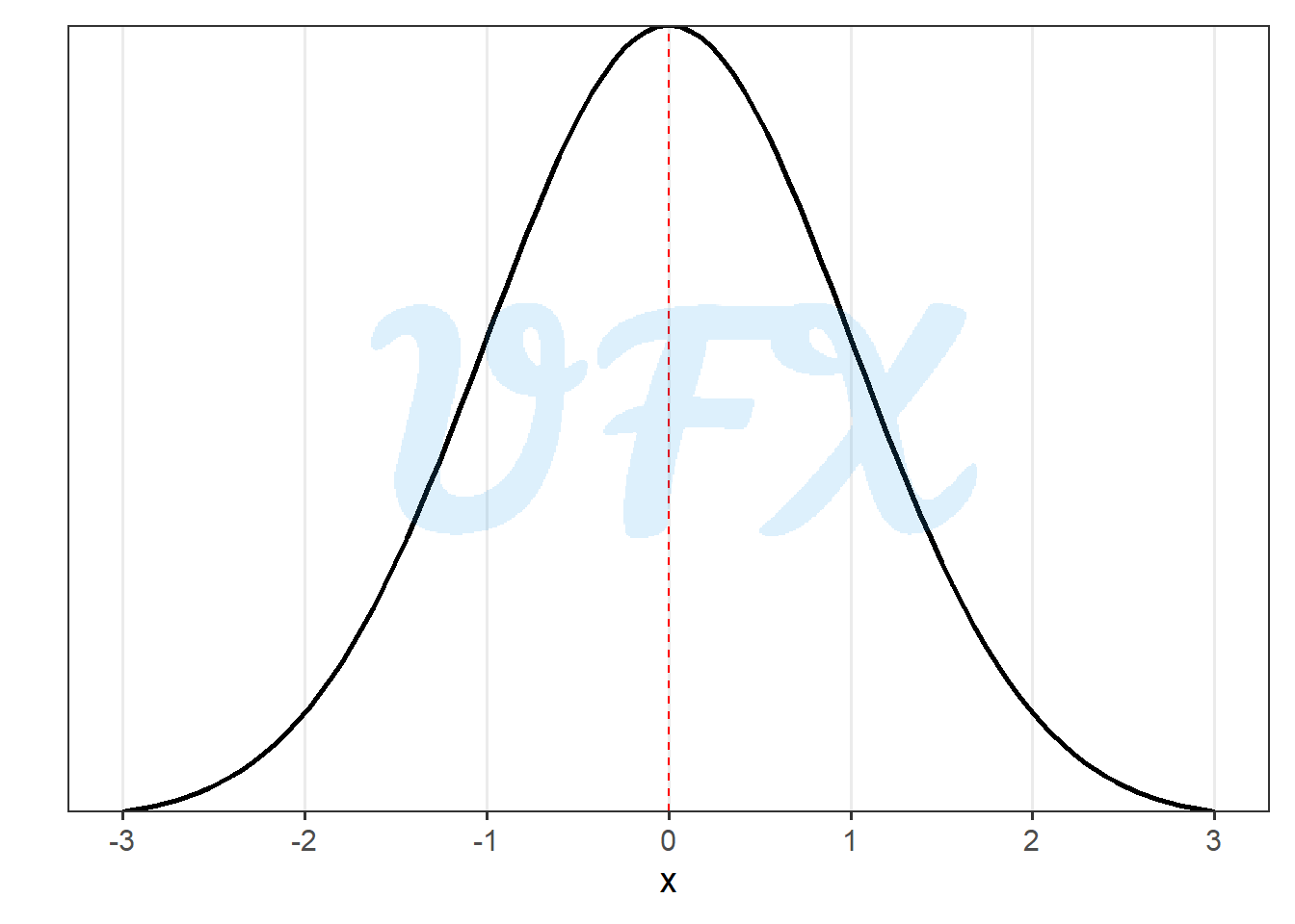
The normal distribution has a balanced and mirror-like shape around its center, which is characterized by its symmetry and central tendency. Because of its symmetry, values on either side of the mean have equal probabilities, and the alignment of the mean, median, and mode at the center.
Here an example of a standard normal distribution:
Bell-shape curve
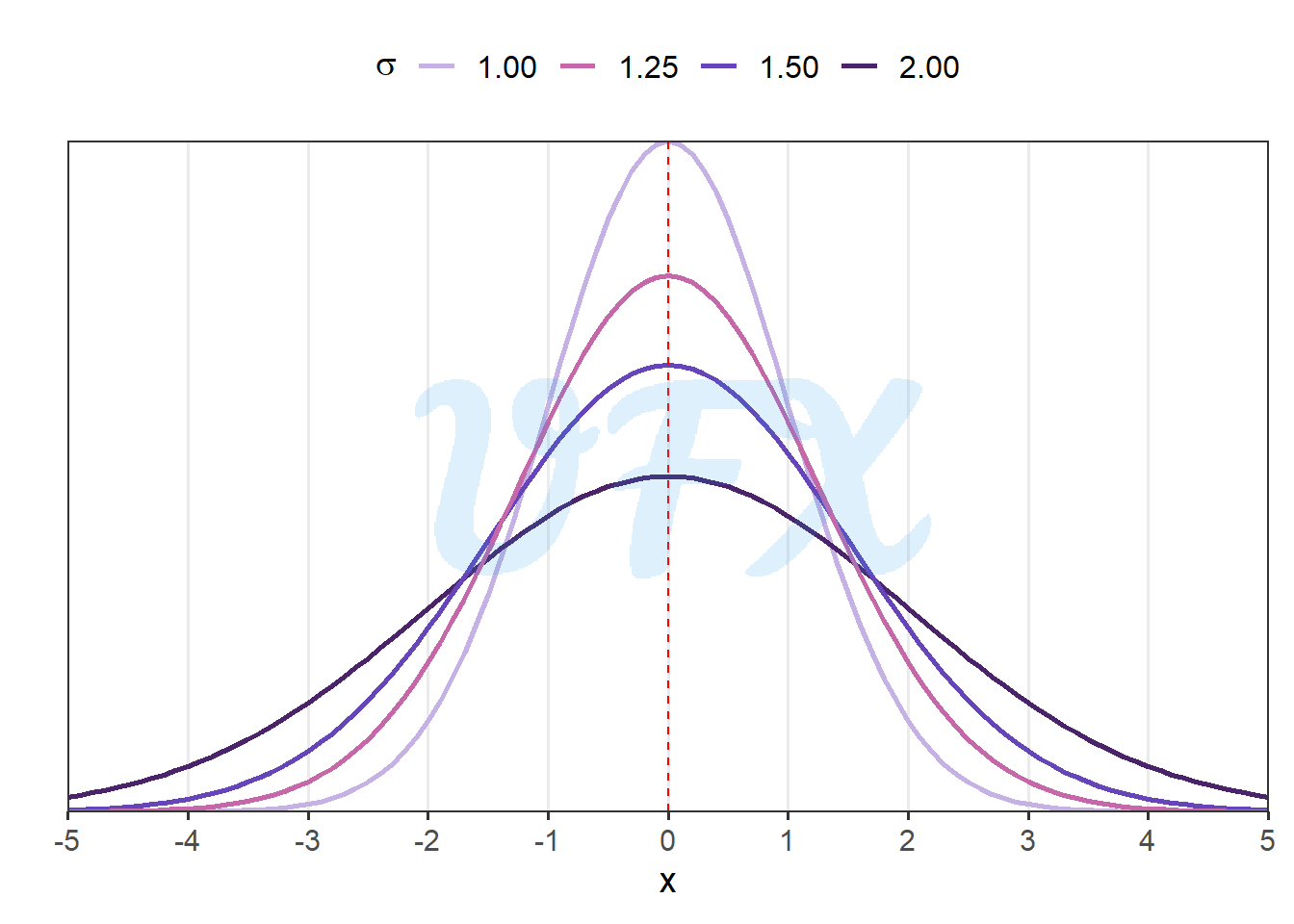
The shape of the normal distribution is also characterized by gradually decreasing probabilities as the values move away equally from the mean in both directions.
Even tough it has zero skewness the variance can imply in a kurtosis change, here a few example:
Chebyshev’s inequality
Chebyshev’s inequality is a mathematical inequality that can be applied to any probability distribution with defined mean and variance. It gives us an bound on the likelihood that a random variable deviates from its mean by a certain amount.
\[ P(|X-\mu| \geq k\sigma) \leq \frac{1}{k^2}, \quad k >0; \quad k \in \mathbb{R}, \tag{3}\]
where:
\(X\) is a random variable with variance \(\sigma^2\) and expected value \(\mu\);
\(\sigma\) is a finite non-zero standard deviation;
\(\mu\) is a finite expected value;
\(k\) is a given real number greater then zero.
When applied to the normal distribution we have that:
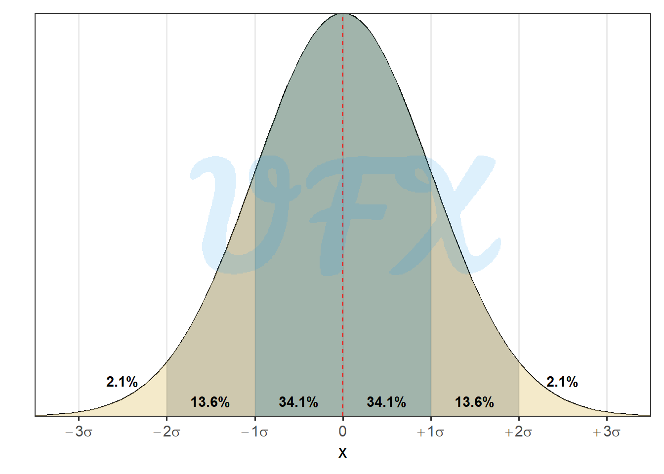
Approximately 68% of values in a normal distribution are within one standard deviation (\(\sigma\)) of the mean, 95% are within two standard deviations, and 99.7% are within three standard deviations.
The Central Limit Theorem (CLT)
According to the CLT, if we combine a large number of independent and identically distributed random variables, the sum will have an approximately normal distribution, regardless of the shape of the original distribution.
For this theorem to work we have three key assumptions for the random variables: independence, identical distribution, and finite variance.
In simpler terms, the CLT allows us to approximate the normal distribution when dealing with large sample sizes and sums of random variables.
A simple application is used in my previous post, where we see that the sum of two dices is approximately a normal distribution.